Rancourt, D.G., Baudin, M., Hickey, J., Mercier, J.
CORRELATION Research in the Public Interest, 17 September 2023
All-cause mortality by time is the most reliable data for detecting and epidemiologically characterizing events causing death, and for gauging the population-level impact of any surge or collapse in deaths from any cause.
Such data can be collected by jurisdiction or geographical region, by age group, by sex, and so on; and it is not susceptible to reporting bias or to any bias in attributing causes of death in the mortality itself
(Aaby et al., 2020; Bilinski and Emanuel, 2020; Bustos Sierra et al., 2020; Félix-Cardoso et al., 2020; Fouillet et al., 2020; Kontis et al., 2020; Mannucci et al., 2020; Mills et al., 2020; Olson et al., 2020; Piccininni et al., 2020; Rancourt, 2020; Rancourt et al., 2020; Sinnathamby et al., 2020; Tadbiri et al., 2020; Vestergaard et al., 2020; Villani et al., 2020; Achilleos et al., 2021; Al Wahaibi et al., 2021; Anand et al., 2021; Bättcher et al., 2021; Chan et al., 2021; Dahal et al., 2021; Das-Munshi et al., 2021; Deshmukh et al., 2021; Faust et al., 2021; Gallo et al., 2021; Islam, Jdanov, et al., 2021; Islam, Shkolnikov, et al., 2021; Jacobson and Jokela, 2021; Jdanov et al., 2021; Joffe, 2021; Karlinsky and Kobak, 2021; Kobak, 2021; Kontopantelis et al., 2021a, 2021b; Kung et al., 2021a, 2021b; Liu et al., 2021; Locatelli and Rousson, 2021; Miller et al., 2021; Moriarty et al., 2021; Nørgaard et al., 2021; Panagiotou et al., 2021; Pilkington et al., 2021; Polyakova et al., 2021; Rancourt et al., 2021a, 2021b; Rossen et al., 2021; Sanmarchi et al., 2021; Sempé et al., 2021; Soneji et al. 2021; Stein et al., 2021; Stokes et al., 2021; Vila-Corcoles et al., 2021; Wilcox et al., 2021; Woolf et al., 2021; Woolf, Masters and Aron, 2021; Yorifuji et al., 2021; Ackley et al., 2022; Acosta et al., 2022; Engler, 2022; Faust et al., 2022; Ghaznavi et al., 2022; Gobiņa et al., 2022; He et al., 2022; Henry et al., 2022; Jha et al., 2022; Johnson and Rancourt, 2022; Juul et al., 2022; Kontis et al., 2022; Kontopantelis et al., 2022; Lee et al., 2022; Leffler et al., 2022; Lewnard et al., 2022; McGrail, 2022; Neil et al., 2022; Neil and Fenton, 2022; Pálinkás and Sándor, 2022; Ramírez-Soto and Ortega-Cáceres, 2022; Rancourt, 2022; Rancourt et al., 2022a, 2022b; Razak et al., 2022; Redert, 2022a, 2022b; Rossen et al., 2022; Safavi-Naini et al., 2022; Schöley et al., 2022; Sy, 2022; Thoma and Declercq, 2022; Wang et al., 2022; Aarstad and Kvitastein, 2023; Bilinski et al., 2023; de Boer et al., 2023; de Gier et al., 2023; Demetriou et al., 2023; Donzelli et al., 2023; Haugen, 2023; Jones and Ponomarenko, 2023; Kuhbandner and Reitzner, 2023; Lytras et al., 2023; Masselot et al., 2023; Matveeva and Shabalina, 2023; Neil and Fenton, 2023; Paglino et al., 2023; Rancourt et al., 2023; Redert, 2023; Schellekens, 2023; Scherb and Hayashi, 2023; Šorli et al., 2023; Woolf et al., 2023).
We have previously reported several cases in which anomalous peaks in all-cause mortality (ACM) are temporally associated with rapid COVID-19 vaccine-dose rollouts and cases in which the start of the COVID-19 vaccination campaign coincides with the start of a new regime of sustained elevated mortality; in India, Australia, Israel, USA, and Canada, including states and provinces (Rancourt, 2022; Rancourt et al., 2022a, 2022b, 2023).
These studies allowed us to make the first quantitative determinations of the vaccine-dose fatality rate (vDFR), which is the ratio of inferred vaccine-induced deaths to vaccine doses administered in a population, based on excess-ACM evaluation on a given time period, compared to the number of vaccine doses administered in the same time period.
The all-ages all-doses value of vDFR was typically approximately 0.05 % (1 death per 2,000 injections), with an extreme value of 1 % for the special case of India (Rancourt, 2022). Our work, using extensive data for Australia and Israel, has also shown that vDFR is exponential with age (doubling every 5 years of age), reaching approximately 1 % for 80+ year olds (Rancourt et al., 2023).
The clearest example is that of a relatively sharp ACM peak occurring in January-February 2022 in Australia, which is synchronous with the rapid rollout of Australia’s dose 3 of the COVID-19 vaccine; occurring in 5 of 8 of the Australian states and in all of the more-elderly age groups (Rancourt et al., 2022a, 2023).
In contrast, often one must contend with the confounding effect of the intrinsic seasonal variation of ACM; however, in this case for Australia, the said January-February 2022 peak occurs at a time in the intrinsic seasonal cycle when one should have a stable (Southern Hemisphere) summer low or summer trough in ACM. There are no previous examples of such a peak in the summer in the historic record of ACM for Australia (Rancourt et al., 2022a).
Few national jurisdictions have the kind of extensive age-stratified mortality and vaccination data available for Australia and Israel. Two other such jurisdictions are Chile and Peru. Here, we show that Chile and Peru, like Australia, has a relatively sharp ACM peak occurring in January-February 2022, which is synchronous with the rapid rollout of Chile’s dose 4 and Peru’s dose 3 of the COVID-19 vaccine, respectively, occurring for all of the more-elderly age groups.
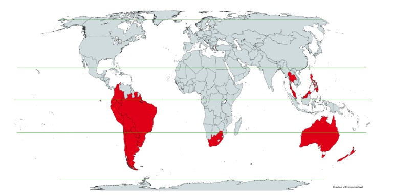
This shared feature between Chile, Peru and Australia led us to look for more examples of the January-February 2022 ACM-peak phenomenon in the Southern Hemisphere and in equatorial regions. Equatorial countries have no summer and winter seasons and no seasonal variations in their ACM patterns. We found the same phenomenon everywhere that data was available (Australia, Bolivia, Brazil, Chile, Colombia, Ecuador, Malaysia, New Zealand, Paraguay, Peru, Philippines, Singapore, South Africa, Thailand, Uruguay), although incomplete for Bolivia and not as distinctive for New Zealand. Here, we report on those findings.
The sources of mortality and vaccine-administration data are given in Appendix A: Sources of mortality and vaccination data.
Appendix B: Examples of all-cause mortality and vaccination data contains examples of the data: all-ages national ACM by time (week or month), from 2015 to 2023, and all-ages all-doses vaccine administration by week, using Y-scales starting from zero, for the 17 countries considered in the present study: Argentina, Australia, Bolivia, Brazil, Chile, Colombia, Ecuador, Malaysia, New Zealand, Paraguay, Peru, Philippines, Singapore, South Africa, Suriname, Thailand, and Uruguay.
Figure 1 shows the said 17 countries considered, in relation to the equator on a world map.
We implement the following method developed by one of us (JH) for detecting changes in regime in ACM data by time (day, week, month, quarter).
One is interested in detecting transitions in time (as one advances in time from a stable historic period) to regimes of “higher than usual” or “higher than recent” ACM, which may be associated with the declaration of a pandemic or with rollouts of vaccines. Although the trained eye can detect such transitions in the raw ACM by time data itself, it is useful to apply a statistical transformation, which is designed to largely eliminate the confounding difficulty of seasonal variations in ACM, which occur in non-equatorial countries.
Since the dominant period of the seasonal variations in ACM is 1 year, and since we wish to detect changes moving forward in time, we adopt the following approach. We apply a 1-year backward moving average to the ACM by time data. Each point in time of the 1-year backward moving average is simply the average ACM for the year ending at the said point in time, and we plot this moving average by time. Changes in regime of ACM then appear as breaks (in slope or value) in the moving average by time.
Note that the 1-year backward moving average method produces one significant but easily discerned artifact: Relatively large and sharp peaks in ACM give rise to artificial drops in the moving average at one year ahead of (later than) the said relatively large and sharp peaks in ACM.
4.1 Historical-trend baseline for a period (or peak) of mortality (Method 1)
Our first method (Method 1) for quantification of vDFR by age group (or all ages) and by vaccine dose number (or all doses) is as follows (Rancourt et al., 2022a, 2023), here improved to adjust for systematic seasonal effects:
- i. Plot the ACM by time (day, week, month) for the age group (or all ages) over a large time scale, including the years prior to the declared pandemic.
- ii. Identify the date (day, week, month) of the start of the vaccine rollout (first dose rollout) for the age group (or all ages).
- iii. Note, for consistency, that the ACM undergoes a step-wise increase to larger values near the date of the start of the vaccine rollout.
- iv. Integrate (add) ACM from the start of the vaccine rollout to the end of available data or end of vaccinations (all doses), whichever comes first. This is the basic integration time window used in the calculation, start to end dates.
- v. Apply this window and this integration over successive and non-overlapping equal-duration periods, moving as far back as the data permits.
- vi. Start each new integration window at the same point in the seasonal cycle as the start of the basic integration window for the vaccine period, even if this introduces gaps between successive integration periods.
- vii. Plot the resulting integration values versus time, and note, for consistency, that the value has an upward jog, well discerned from the historic trend or values, for the vaccination period.
- viii. Extrapolate the historic trend of integrated values into the vaccination period. The difference between the measured and extrapolated (historic trend predicted) integrated values of ACM in the vaccination period is the excess mortality associated with the vaccination period.
- ix. The extrapolation, in practice, is achieved by fitting a straight line to chosen pre-vaccination-period integration points.
- x. If too few points are available for the extrapolation, giving too large an uncertainty in the fitted slope, then impose a slope of zero, which amounts to using an average of recent values. In some cases, even a single point (usually the point for the immediately preceding integration window) can be used.
- xi. The error in the extrapolated value is most often overwhelmingly the dominant source of error in the calculated excess mortality. Estimate the “accuracy error” in the extrapolated value as the mean deviation of the absolute value difference with the fitted line (mean of the absolute values of the residuals) for the chosen points of the fit. This error is a measure of the integration-period variations from all causes over a near region having an assumed linear trend.
- xii. The said “accuracy error” is generally larger than the “precision error” (or statistical error) in the extrapolated value, as it represents the year-to-year variability of the integrated ACM in the integration window in the years prior to the Covid or vaccination periods.
- xiii. If there are too few integration windows in the available normal years prior to the peak or region of interest to obtain a good estimate of the historic year-to-year variability, or if the statistical errors in the integrated values are relatively large, then make use of the statistical errors to best estimate the needed uncertainty.
- xiv. Apply the same integration window (start-to-end dates during vaccination) to count all vaccine doses administered in that time.
- xv. Depending on particular circumstances in the data, it may be necessary to use different integration bounds (different windows) for the ACM and for the vaccine administration. We saw no need for this, and we did not try to implement or test such an optimization.
- xvi. Define vDFR = (vaccination-period excess mortality) / (vaccine doses administered in the same vaccination period). Calculate the uncertainty in vDFR using the estimated error in vaccination-period excess mortality.
The same method is adapted to any region of interest (such as a peak in ACM) of sub-annual duration, by translating the window of integration (of the region of interest) backwards by increments of one year.
The above-described method is robust and ideally adapted to the nature of ACM data. Integrated ACM will generally have a small statistical error.
A large time-wise integration window (e.g., for the entire vaccination period) mostly removes the difficulty arising from intrinsic seasonal variations; and this difficulty is further solved by starting each new integration window at the same point in the seasonal cycle as the start of the basic integration window for the vaccine period (point-vi, above).
The historic trend is analysed without introducing any model assumptions or uncertainties beyond assuming that the near trend can be modelled by a straight line, where justified by the data itself. Such an analysis, for example, takes into account year to year changes in age-group cohort size arising from the age structure of the population. The only assumption is that a locally linear near trend for the unperturbed (ACM-wise unperturbed) population is realistic.
While the above method is designed for cases (jurisdictions) in which there is no evidence in the ACM data for mortality caused by factors other than the vaccine rollouts, such as Covid measures (treatment protocols, societal impositions, isolation and so forth; since no excess mortality occurs in the pre-vaccination period of the Covid period), it can be readily adapted to cases in which mortality in the vaccination period is confounded by additional (Covid period) causal factors that cannot be ruled out.
One approach is simply to adapt the above method to calendar years, irrespective of whether excess mortality occurs prior to the COVID-19 vaccine rollouts. One obtains excess ACM by calendar year, relative to the expected value from the historic trend deduced by linear extrapolation from a chosen range of yearly ACM values for < 2020 (for years prior to 2020, when the 11 March 2020 announcement of a pandemic was made). One then compares the excess ACM for 2020 and for 2021. In many (most) countries, there was essentially no COVID-19 vaccination in 2020, and a rapid rollout essentially started in January 2021.
4.2 Special Case of a Single Historic Integrated Point (Method 2)
In cases in which it is not possible or practical to obtain more than one integration value for the needed extrapolation (steps v to ix, above), rather than assume a zero slope for the extrapolation (step x, above), the following second method (Method 2) can be applied.
If Y(-1) is the sole historic integrated point, then simply take the needed extrapolated value, Y(0), to be:
| Y(0) = Y(-1) + m ΔT W | (1) |
where m is the slope of the best-straight-line fit through the original ACM by time unit (day, week, month…) versus numbered time unit, ΔT is the number of time units between Y(0) and Y(−1) (i.e., between the start of the Y(0) integration window and the start of the Y(−1) integration window), and W is the inclusive width of the integration window in number of time units.
This assumes that the ACM by time varies on a straight line, notwithstanding seasonal variations, on the near segment used to obtain the best-straight-line fit.
The resulting excess mortality for the integration window or period, xACM(0), is then:
| xACM(0) = ACM(0) - Y(0) | (2) |
where ACM(0) is the integrated ACM in the period of interest.
The statistical error (standard deviation) in xACM(0) is then given by:
| sig(xACM(0)) = sqrt [ ACM(0) + Y(−1) + (ΔT W sig(m))2] | (3) |
where sig(m) is the nominally statistical error in m.
If there is no seasonal variation in ACM, as occurs in equatorial-latitude jurisdictions, then sig(m) is the actual statistical error in m. With seasonal variations in ACM, sig(m) extracted from the least squares fitting to a straight line does not have a simple meaning. In this case, sig(m) will incorporate uncertainty arising from seasonal variations, and increases with increasing amplitude of the seasonal variation.
4.3 Application of the Methods to the Specific Countries
The parameters for applying the methods (Methods 1 and 2) to the data are given in Appendix C: Technical and specific information for applications of the methods to the data.